Multiphysics reduced order model
:hourglass: 30 min read. :rotating_light: An advanced topic. :heart: A topic that I really like!
Highlights
- Situation
- Task
- Action
- Result
The business goal
Simulations is the super-power that engineers use to reduce costs, mitigate risks and improve performance of their products. The holy grail is to run simulations fast; not just faster, it needs to be as fast as real-time. This means the delivering target is 60-90 frames per second without compromising the accuracy. Before the “big data”, “AI” and “neural networks” came into play, the only method to achieve real-time simulations was with reduced order models (ROM). Netural nets bring is ease of use because reduced models are admittely harder to formulate. What you get in return however is more confidence on the accuracy, for example with reduced order models there is no guess on the architecture of the netural net. With ROM all remains rigorous and measuable.
There is another dimension to the complexity: the real-life problems that we want to simulate are complex in nature because many physics play a role concurrently. These are multiphysics problems. Comsol and Physica, respectively developed at KTH and from Swansea univeristies, were the first codes offering multiphysics solutions. Today the landscape is very different and the vast offering of solutions can be seen as a demonstration of the major technical challenges involved.
Being able to identify the method that gives the right solution in a timely manner is the key to stay ahead of the game. This is what the business wants, and in what follows I’ll expand on technical details that are important to take informed (business) decisions.
The Method
We’ll be looking at the formulation of ROM of multiphysics problems, coupling computational fluid dynamics (CFD) and thermo-dynamics. In other words, we’ll be coupling heat and mass transport problem. Our ROM will be based on Proper Orthogonal Decomposition and Galerking projection. Propert Orthogonal Decomposition (POD) is the we method used to compute the trial functions of the Galerking project that we’ll call modes. Next, we’ll move quickly from the strong form to the weak form of the PDE.
Strong form
The strong form of the heat and mass transfer problem comprises few equations: Continuity, Navier-Stokes and Boussinesq approximation.
$$ \left \{ \begin{matrix} \rho ( u_{i,t} + u_{j} u_{i,j} ) & = &\sigma_{ij,j} + f_i \\ \rho c_p ( \theta_{,t} + u_{j} \theta_{,j} ) & =& k \theta_{,jj} \\ u_{i,i} &= &0\\ \end{matrix} \right. $$
Yes, we are assuming incompressible fluid. Also, we need to add two quations to describe the stress as a function of velocity $u$ and the buoyancy forces as a function of the temperature $\theta$:
$$
\begin{matrix}
f_i & = & \beta ( \theta - T_{\infty} ) g_i \\
\sigma_{ij,j} & = & -p \delta_{ij} + \mu ( u_{i,j} + u{j,i} ) \\
\end{matrix}
$$
How about boundary conditions? Of course we need them and we’ll consider very general cases:
$$
\begin{matrix}
u_i = G_i(x) & \text{and} &~ \theta = T_0(x) & \text{on} & \Gamma_D ~ \forall ~ t \\
\sigma_{ij} ~ n_j = 0 & \text{and} &~ \frac{\partial \theta}{\partial \mathbf{n}} = F_0(x) & \text{on} & \Gamma_N ~ \forall ~ t \\
\end{matrix}
$$
All the new quantities introduced in the last two equations are known and, if you’ve made it this far in the article, they should make sense to you. Note that these are not zero - it would have been much easier if considered them homogenous. For initial conditions however zero or not-zero makes not difference.
The one thing making POD-based formulation hard
I’ve probably lost more of the readers by now and before you leave too I wanted to explain why I wrote that reduced models are a difficult topic to graps. As we move toward the weak formulation of the multiphysics problem we have to approximate our unknown fields, and that’s we the complexity begins. We are going to split the unknowns into fields comprised of two fields: a known reference field and an unknown homogenos field. That’s easy, but if our strong form had about 10 terms, our weak form it’s now going to have twice as many… scale up to a 3D problem and the actual terms to compute become 50 or so. I’m actually to lazy to count but that’s why we have no other option than using the index notation - if you wondered why :nerd:.
We’ll start from the temperature because is a scalar field and makes things easier:
$$ \theta(\mathbf{x},t) = R\theta(\mathbf{x},t) + H \theta(\mathbf{x},t) $$
I’ve specified that the temperature varies in time and space $\theta(\mathbf{x},t)$ just to highlight this fact. I have also splitted the temperature field into two: a reference field $R\theta$ and an homogenous field $H\theta$. The latter is defined such that all its essential (or Diriclet or explicit) boundary contidions are zero. That’s not physical, but that’s what it is and the worst has yet to come: $R\theta$ is actually arbitrary expect it must satisfy the essential boundary conditions of the original problem, that is $T_0(x)$ on $\Gamma_D$. This is when we lose contact with the physics we are most familiar with the reason for writing the unknown field in this way will become evident later on.
Now the separation of variables for the temperature filed:
$$ R\theta(\mathbf{x},t) = RT(\mathbf{x}) ~ \dot{h}(t) $$ $$ H \theta(\mathbf{x},t)=\sum^e_{c=1} \phi^c(\mathbf{x}) ~ \omega^c(\mathbf{t}) $$
If you read a paper on reduced modelling and they solve a homogenous problem you don’t see the reference field and its components, which are indeed not so important. All they need to do is to fulfil the essential boundary conditions of the original problem. From here it follows that no matter what shape we give to $RT(\mathbf{x})$, the boundary conditions must apply to $\dot{h}(t) ~ \forall ~ t$. The homogenous part is more interesting is the linear combination of the modes $\phi^i(\mathbf{x})$ with the reduced model’s unknowns $\omega^i(\mathbf{t})$. The modes are a series of structures defined over the domain and the unknowns are their coefficients that vary in time.
To wrap up this section I’ll put down in words what’s the one thing making POD-based formulations so hard. You may have guessed already, but when you combine the last three equations you’ll have two not-so-common terms describing the temperature field. To these add the velocity’s equivalent: each velocity’s component will also be described by two not-so-common terms, leading to $2 \times 3 = 6$ terms for 3D problems. Substitute these $8$ terms in the strong form and the governing equations will look like this: For the temperature:
$$
\begin{matrix}
RT ~ \dot{h} &+& \left ( \dot{m}\dot{h} - \frac{k}{k_{ref} \dot{h}} \right ) RT_{,j} RU_j + \dot{m} RU_j \phi^c_{,j}\omega^c + \\
& +& \dot{h} RT_{,j} \varphi^l_j \alpha_l + \phi^c \omega^c_{,t} +\phi^c_{,j} \varphi^l_j\alpha^l \omega^c - \frac{k}{\rho c_p} \phi^c_{,jj} \omega^c &= 0
\end{matrix}
$$
If you read all that aloud take a long breath now because here it comes the one for the velocities terms:
$$
\begin{matrix}
RU_i ~ \dot{m} &+& \varphi^l_i \alpha^l_{,t} + \dot{m} RU_j \varphi^l_{i,j} \alpha^l + \dot{m} \varphi^l_j RU_{i,j} \alpha^l + \\
& +& \varphi^l_j \varphi^m_{i,j} \alpha^l \alpha^m + \left ( \dot{m} - \frac{k}{k_{ref} \dot{m}} \right ) \frac{RP_{,i}}{\rho} - \frac{\nu}{\rho} \varphi^l_{i,jj} \alpha^l + \\
& -& \frac{\nu}{\rho} \varphi^l_{j,ij} \alpha^l - \beta_{ref} \left ( \dot{h} RT + \phi^c \omega^c - T_\infty \right ) g_i + \frac{1}{\rho} \psi^q_{,i} \varepsilon^q &= 0
\end{matrix}
$$
I’d expect at least few typos in there, but if you look closely for a more genuine reason you’ll also find nonlinear terms. They come from the Navie-Stoks of course, but now instead in the velocity are in the corresponding reduced model’s variable $\alpha$. In all the above repeated index means summation, i is the for the i-th velocity component, $RP$ is the reference field for the pressure and similarly other constants $\cdot_{ref}$. Oh, I forgot $\psi^q$ are the pressure modes. That’s all folks.
About the modes
They come from the proper orthogonal decomposion (POD). To get the modes you have to solve a singular value decomposition problem and hope that all comes out positive defined. Actually, if you’re using Matlab you also have eigs coolest function ever with lower memory footprint than eig. Yeah, the caveat is the approximation on the modes, but that’s acceptable. Go for it and tell your supervisor I told you!
By definition all models are orthogonal which means that the mass matrix of your reduced system will, in the end, be diagonal. But to see that you really have get to the end 😈.
Modes. Modes for fluid and modes of heat.
I thought some pictures would please your eyes. Here you can admire the shape of fluid’s velocity and heat. These are the particular model for a fluid flow past a cyliner - a very standard problem Google can tell you more about. The modes are static but when combined toghether they can produce the eddis and even the thermal field. Majastic!
Here’s how the modes look like. Hopefully you can see that the blue-ish are for the flud and the orange-ish are for the heat field and in all these pictures the cylinder is..well..the cylinder of the fluid flow past a cyliner problem Google told you about.
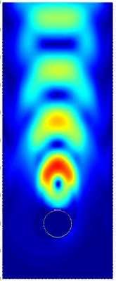
Velocity modes
The modes are all different. They have “frequencies” that increase as you look left to right. And they look fabolous. If you want to produce fabolous pictures of modes too, you’ll have to run a full CFD simulation and extract snapshots from there. I reccomend the paper from H. M. Park and M. W. Lee, ‘An efficient method of solving the Navier–Stokes equations for flow control’, International Journal for Numerical Methods in Engineering, vol. 41, no. 6, pp. 1133–1151, 1998.
Now repeat close your eyes are repeat.
All data and no play makes model a dull model
All data and no play makes model a dull model
All data and no play makes model a dull model
All data and no play makes model a dull model
… did you not see Shining?! Did you not see that POD trains the model with data?! Over-abused terms in this day an age, but that’s really what it’s all about here: modes limit the solution space and allow reduced models be fast and accurate.
If you where to do this with neural nets you’d need a GPU, tons of Python packages you don’t know how to use and you have to come up with an architecture of a neural net. With reduced model you need an SVD solver. By the time your mate installs Tensors Flow you’ll get the training done.
As in with neural nets, your model will become dull as soon as you depart significantly from the training data or if you simply scre up the sampling of the snaptshot method. Don’t screw up the sampling, please.
Final stretch to the weak form
to be continued…. Admittedly, I got carried away with the many equations, but I’ll complete this article by Christmas (2021) ;).