Hands-on reduced order modelling

⌛ 15 min read.

First date with reduced order modelling? Here’s what it is

When it comes to explain what is reduced order modelling, this Wikipedia page gets really close to perfection:

Reduced order modelling is a technique for reducing the computational complexity of mathematical models in numerical simulations.

I like this definition because reduced order modelling is just about that really! There are no assumptions about the physics, nor expensive GPUs to heat up our planet behind the scene. Loosely speaking what’s reduced is the mathematical space in which we seek the solution. The reduction of the complexity translates into a reduction of computing time not factor 2x or 5x, but at least 100x!

The math behind this technique is rigorous but can be hard to grasp. Perhaps because reduced order modelling is not mainstream yet, it is not taught widely, and currently there still is a lot of research ongoing. Still, the early results are terrific and once the math ‘clicks’ into your brain, all becomes incredibly interesting and really fascinating. Let’s see if I can pass some on that amusement to you as well.

Before moving on, what I don’t like about the Wikipedia’s definition? Reduced order modelling is a family of techniques. It’s a large and growing family by the way, which reflect the fact that we’re only seeing the tip of the iceberg that researchers will produce in the near future!

Put your hands on it

Having a math or engineering degree would help you to understand that the key behind reduced modelling there are two key concepts: (i) modes and (ii) that a function can be interpolated with:

$$ u(x,t) = \sum_{i=1}^n N(x)_i V_i(t) $$

But if this means nothing to you, here’s essence of modes and interpolation. First, a mode can be seen as a typical pattern of a system. Modes have shape and frequency. For example, a bottle full of water when turned upside down drains, and as it does so, bubbles of air find their way into the bottle to compensate for the water dropping on your floor. The frequency of those bubbles of air is pretty much consistent if you empty dozens of water bottles. The sound the bottle makes in the process is also pretty consistent, indicating that the shape of the sound waves is consistent. That’s just an example about the shape and frequency of modes.

Now interpolation. You can approximate a very complex function $u(x,t)$ in two variables, in this case $x$ and $t$, with many simple functions, such as $N(x)_i$ and $v_i(t)$. That’s what finite element does by the way. And after reading the inspiring book Approximation Theory and Practice by Prof. Trefethen I cannot tell the difference between interpolation and approximation — at least in our context. So, in more general terms, we want to approximate a function in two or more variables, with many simple functions that have only one variable. One variable only, this is very important and is known as separation of the variables. It basically allows to decouple whatever happens in our system into functions that are independent of one another. Take the example $u(x,t)$, if $x$ is space and $t$ is time, we will use $n$ functions $N(x)_i$, that vary only in space, and pair them up with $n$ functions $V_i(t)$, that vary only in time, to reduce-model an impact!

Reduced order modelling for a simple impact test

I will present an impact problem I’ve solved using LS-DYNA. Yes, I do work at ANSYS, but I’m not writing this blog to endorse or promote any product. This work goes back to 2018, while I was at Oxford and LS-DYNA was not even part of ANSYS. I believe LS-DYNA was one of the first widely used commercial codes to implement some basic capabilities for reduced modelling, so here we are.

The model comprises a blade and rather large conic projectile. The geometry, the coarse and the fine meshes used are these below:

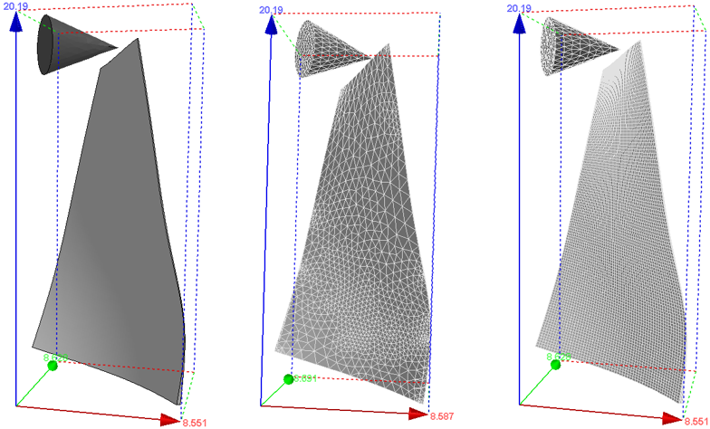
The projectile has a certain initial velocity, hits the tip of the blade and that’s it. Very simple. With classic finite element analysis, this model would have at least 2000 nodes, easily 50000. Each node would have 3 degrees of freedom, but with reduced modelling you can expect really good results with 100 degrees of freedom.

LS-DYNA is limited in the sense that can only work with free vibration modes, but other methods based on snapshots would lead to a much more powerful reduced model. I would recommend reading the paper by Parks and Lee [1] for the method of snapshots. For LS-DYNA one of the few references published is the paper by Maker and Benson [2]. This paper describes step by step how to extract the modes and setup the reduced model for the impact analysis, so I will not duplicate the content. Instead, I’ll present some results below.

---

Results - writing in progress :)

I’m on it, just need a bit of time to write up this last part. Come back soon!

s	FEA elements	ROM modes
Number of nodes	2110, 32205	30 , 90

Number of CPUs 2 1 2 1 1 CPU time (min) 500 5 831 37 64

References

[1] H. M. Park and M. W. Lee, ‘An efficient method of solving the Navier–Stokes equations for flow control’, International Journal for Numerical Methods in Engineering, vol. 41, no. 6, pp. 1133–1151, 1998.

[2] B. N. Maker and D. J. Benson, ‘Modal methods for transient dynamic analysis in LS-DYNA’, in 7th International LS-DYNA Conference, 2002.

[3] J. Fehr, P. Holzwarth, and P. Eberhard, ‘Interface and model reduction for efficient explicit simulations - a case study with nonlinear vehicle crash models’, Mathematical and Computer Modelling of Dynamical Systems, vol. 22, no. 4, pp. 380–396, Jul. 2016.