Create solid NURBS with Matlab
:hourglass: 10 min read. :bulb: 5 min coding
Unlock isogeometric analysis by hand-crafting solid NURBS (trivariate) with Matlab.
What is isogeometric analysis?
There are tons of good references out there to answer this question, but here I’m taking the perspective of a mechanical engineer that designs components and uses FEM to validate the mechanical properties. For most engineers this is the standard procedure: draw a concept design into a CAD software, make it simpler by removing details unecessary for the analysis, mesh the component(s) and finally run the FEM analysis.
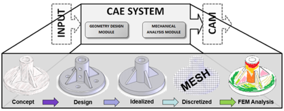
Standard workflow used in mechanical engineering for designing all sort of components.
Meshing is a detious, time consuming and yet terribly important step of this process. The main idea of isogeometric analysis (IGA) is to take the costs of meshing out of the equation. That is, at least in principle, what drives today’s research.
Learn to learn
You must be solid on the math behind NURBS. Personally I started from Wikipedia and dived deeper into The NURBS Book. I created matlab scripts to create all plots of the first 5 chapters of that book using mostly built-in functions.
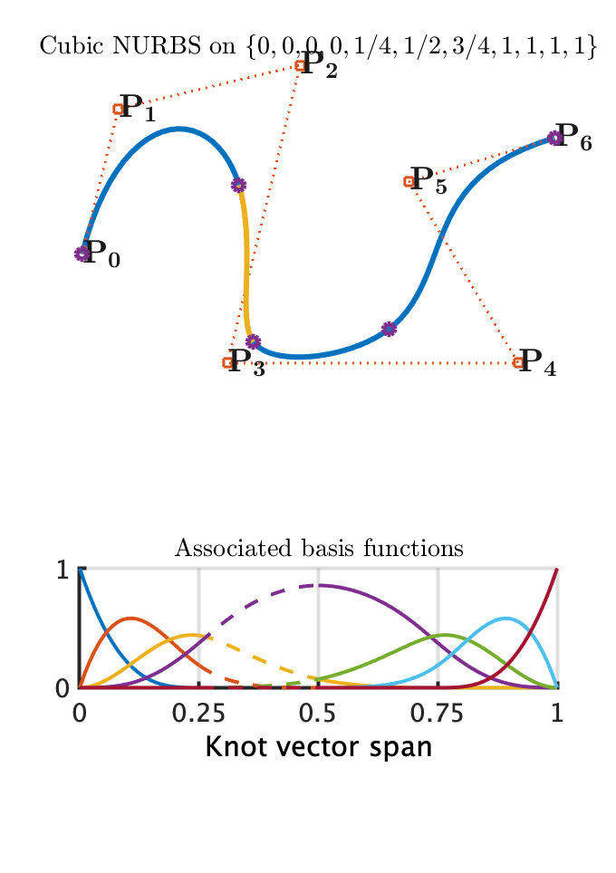
This is the script I created to plot Figure 4.1 - shown below.
KnotS = [0 0 0  0 1/4 1/2 3/4 1 1 1 1];
% Control polygon and weights
x = [0    0.2500    1.5000    1.0000    3.0000    2.2500    3.2500];
y = [0    1.0000    1.3000   -0.7500   -0.7500    0.5000    0.8000];
z = [0         0         0         0         0         0         0];
w = [1         1         1         3         1         1         1];
% Assmble coefficients and nurbs
HomCoef = [x.*w;y.*w;z.*w;w];
rs = rsmak(KnotS, HomCoef);
figure
% Plot curve
    subplot(2,1,1);
        hold all, axis tight equal; grid on
        fnplt(rs)
    % ...and a part of segment
        fnplt(rs,KnotS([5 6]),3)
    % ...and the points on the curve
        vals = unique(fnval(rs,KnotS)','rows')';
        plot3(vals(1,:),vals(2,:),vals(3,:),...
            'o','markersize',6,'linew',3)
% Plot basis functions in intervals
    subplot(2,1,2) ; hold all
        axis tight equal; grid on
        BasFuncts = rsmak( KnotS, [eye(rs.number).*repmat(w,size(x,2),1);w]);
    % ...the first interval
        PlotInterval = 0:.01:KnotS(5);
        vals = fnval(BasFuncts, PlotInterval);
        plot(PlotInterval,vals.','-','linew',2);
    % ...the second interval
        PlotInterval = KnotS(5):.01:KnotS(6);
        vals = fnval(BasFuncts, PlotInterval);
        plot(PlotInterval,vals.','--','linew',2);
    % ...and the last interval
        PlotInterval = KnotS(6):.01:1;
        vals = fnval(BasFuncts, PlotInterval);
        plot(PlotInterval,vals.','-','linew',2);
Trivariate Solid Cylinder
The LS-Dyna card for this example can be downloaded from here. It simply consists of solid rod, represented by a single NURBS patch. In my paper I discussed all details of this problem but this is also the simplest shape I created in Matlab.
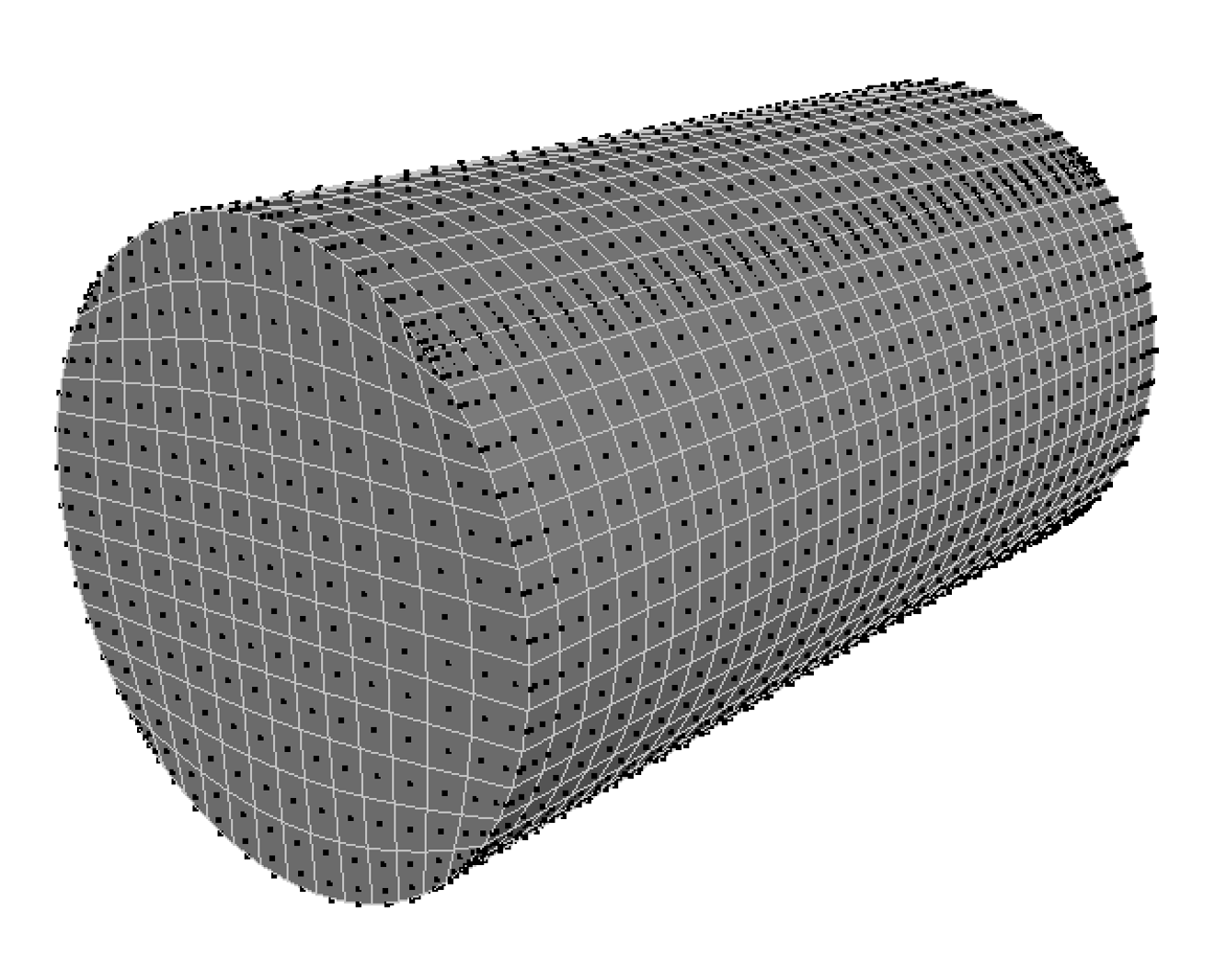
Solid rod as a single NURBS patch.
Start off by declaring the order in each of the three parametric directions and the number of control points associated to them:
% Basic geometry NURBS parameters
% ... its order
PU = 2;
PV = 2;
PW = 1;
% ... its number of control points
NPU = 3;
NPV = 3;
NPW = 2;
Create a general distribution of control points in space:
% Generate NURBS control grid
[XU,YV,ZT] = meshgrid(  linspace( -L  ,  L  , NPU),...
                        linspace( -L  ,  L  , NPV),...
                        linspace(-H/2 , H/2 , NPW));
and the know vectors:
% Compute knot vectors
KnotU = augknt( linspace(0,1,PU+1+NPU-2*(PU+1)  + 2 ),PU+1);
KnotV = augknt( linspace(0,1,PV+1+NPV-2*(PV+1)  + 2 ),PV+1);
KnotW = augknt( linspace(0,1,PW+1+NPW-2*(PW+1)  + 2 ),PW+1);
Now you need to loop over the longitudinal direction to modify the position of the control points.
for iX = 1 : NPW % Loop over the layers in W-direction
    iStat = (iX-1) * NPU*NPV;
    % Number of points in the current countr
    NumPerEdge = NPV - 2*(1-1);
    % Nodes' ids on current layer - this could be improve/generalised
        id = [ (1:NumPerEdge) + (1+NPU)*(1-1), ...
             [NumPerEdge+1:NPU:NumPerEdge*(NumPerEdge-1)]+ (2*NPU)*(1-1),...
             [2*NumPerEdge:NPU:(NumPerEdge-1)*(NPU)]+(NPU)*(1-1),...
             [(NPU-1)*NumPerEdge+1:NumPerEdge*NPU]+ (NPU-1)*(1-1)];

    id =id + iStat;

    % Adjust coordinates to create a perfect circle
    XU( id([2 4 5 7]) ) = XU( id([2 4 5 7]) ) .*2;
    YV( id([2 4 5 7]) ) = YV( id([2 4 5 7]) ) .*2;
end
Setting all weights of all control points tosqrt(2)/2 is the first step we need to do before creating the NURBS object. For simplicity, it’s also useful to readjust the coefficients of the NURBS:
% Assemble coefficients into NURBS structure
    % ... Control poins
    x = XU(:); y = YV(:); z = ZT(:);
    % ... Coeff. for rsmak
    Coef = zeros([4,size(XU)]);
    Coef( 1,1:NPU,1:NPV,1:NPW) = reshape(x,1,NPU,NPV,NPW) .* reshape(w,1,NPU,NPV,NPW) ;
    Coef( 2,1:sNPU,1:NPV,1:NPW) = reshape(y,1,NPU,NPV,NPW) .* reshape(w,1,NPU,NPV,NPW) ;
    Coef( 3,1:NPU,1:NPV,1:NPW) = reshape(z,1,NPU,NPV,NPW) .* reshape(w,1,NPU,NPV,NPW) ;
    Coef( 4,1:NPU,1:NPV,1:NPW) = reshape(w,1,NPU,NPV,NPW) ;
wherewsimply is a vector of weights for all control points.
We can finally execute the lines that accutally return a solid NURB:
NURBS = rsmak({KnotU,KnotV,KnotW} , Coef );
The content of the matrixCoefis just what described above and is a collection of all control points’ coordinates divided by the respective weights. The best place to read about this is Matlab’s documentation on thersmakfunction.
Visualisation
Of course it would be nice to visualise the NURBS in Matlab before going in LS-Dyna. Unfortunately the functions built-in are limited, butfnpltis a good starting point to create your own.
I created a modified version offnpltthat takes the same input parameters of standard 3D visualisation commands, likesurf. Just typeedit fnplt and you can easily editnpointsto change the resolution of the image rendered by Matlab. After a long time practising and improving my scripts I created and rendered a dogbone specimen geometry using solid NURBS. Following this prodedure I also crated a ballistic impact model for LS-Dyna.
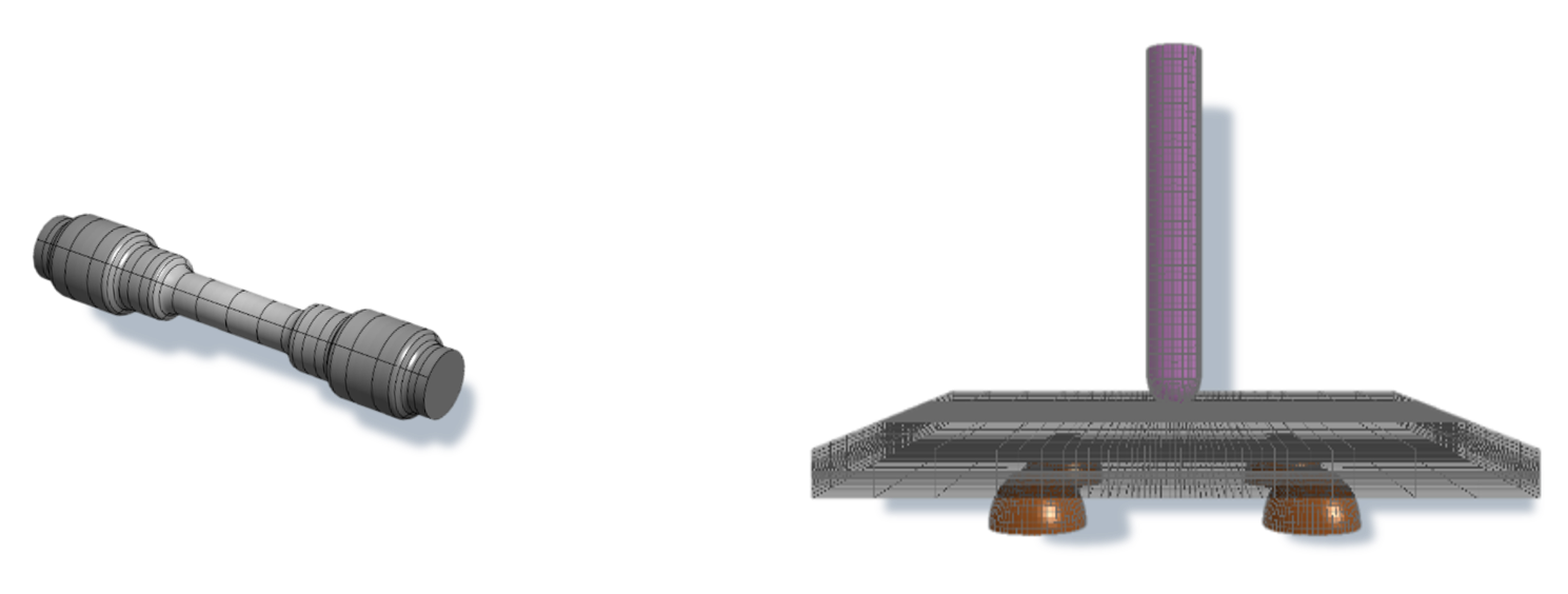
I’d conclude by saying that if you do have time you can create simple models and run in LS-Dyna IGA to discover where FEM shows major limitations.
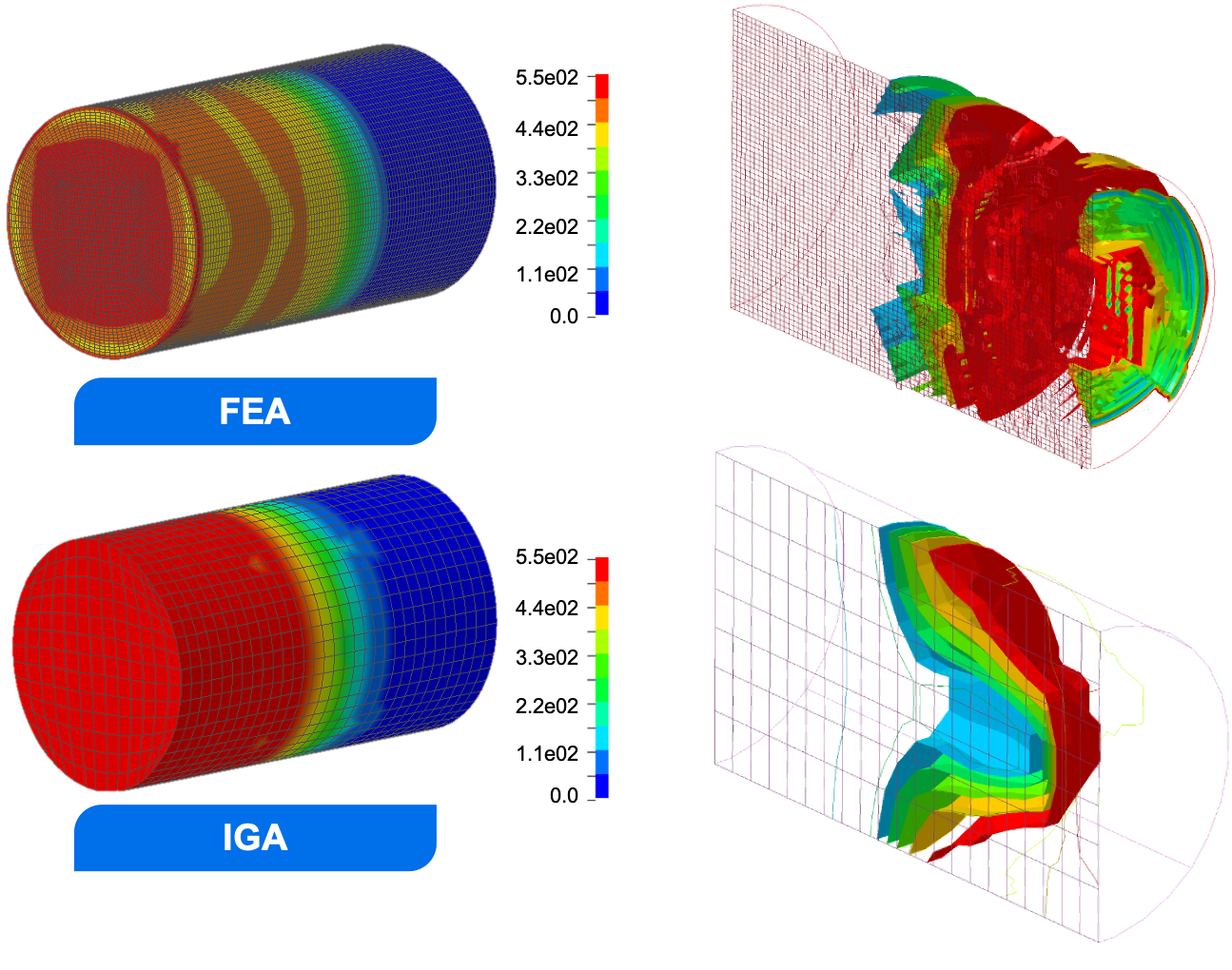
By comparing the stress wave propagation in a solid rod by FEM and IGA, a striking result is the different shapes of the fron wave at its highest value (red isosurface).
Complex shapes from a CAD geometry
Since 2013 I worked with the developers of LS-Dyna to explore what IGA can do and the first barrier was, surprisingly, building a solid model. While in FEM you need a mesh, in IGA you need a trivariate NURBS and that’s not something easy to create.
What I created was simply toolbox to generate single-patch trivariate NURBS out of CAD models. The models below show the various steps for the model of a turbine blade. The optimsation is not really rigorous and needs tweaks, but does the job for what I wanted to do: run an IGA model in LS-Dyna. Mode details on this are in three papers I published with colleagues from Livermore, what I want to focus here is the backend library in Matlab.
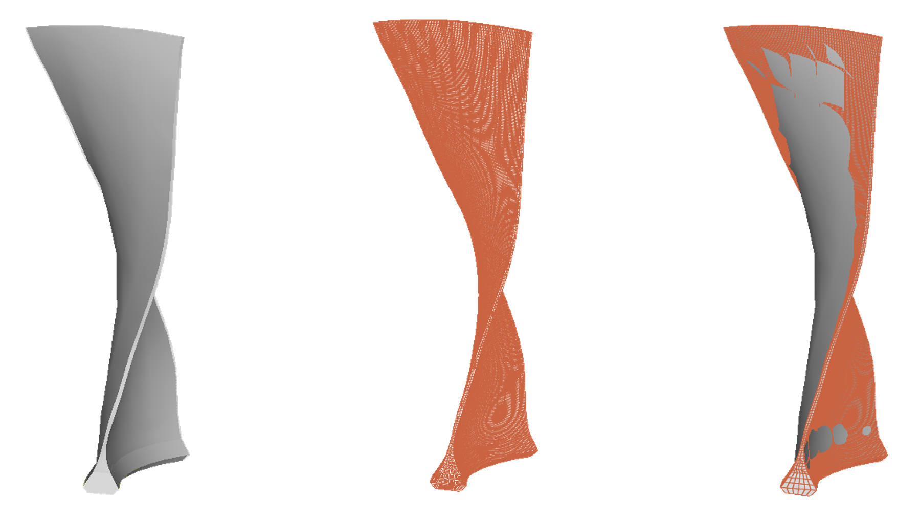
Take a CAD model (left), mesh it as it is (center) and optimase the shape of a trivariate NURBS to match the mesh nodes.
Since I created this rudimentary toolbox LS-PrePost and many other NURBS libraries became avaiable. If that’s where you start from, I’d reccomend looking at SISL and pyNURBS.